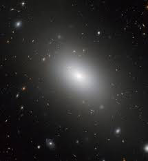
An elliptical galaxy

This programing exercises is designed to help you to become  familiar with how to make some basic plots and carry out some simple statistical analysis with simulation data. The goal is to gain experience with programing in IDL, Python or Fortran (with pgplot). Currently (in 2019) you are strongly encouraged to use Python. I strongly recommend installing Python and Jupyter using the Anaconda Distribution, which includes Python, the Jupyter Notebook, and other commonly used packages for scientific computing and data science (e.g. Numpy, MatPlotLib, scipy). You may want to also download the astropy library.

First download this coorda_exercise.zip file and unpack it (it should download and automatically unpack on a Mac). The directory contains the following 3 files:

1. A data file coordAa.dat.txt: This file is an ASCII data file that contains positions and velocities  (also called “phase-space coordinates”) in Cartesian coordinates (x, y, z, vx, vy, vz) for around 40,000 particles representing “stars” in an elliptical galaxy sort of like this one. But the data file contains a simulation – which means each “star” in the simulation is actually the mass of many many stars (below you are asked to figure out how massive each star is).
2. A README file called Coorda_Exercise_README.txt:  which contains some instructions on how to run Jupyter notebooks. Read this!
3. A Jupyter (python) notebook file called galaxy_exercise.ipynb: This will look completely unintelligible if you open it with a text editor but don’t be alarmed! This starter Jupyter notebook will set you on your path to scientific programing. You can use to read the data file  coordaA.dat.txt and  to start making cool plots. The first few steps of the exercise are already done in this notebook.

Here is the exercise you are asked to complete.

1.  Learn how to read in the data from the ASCII file coordaA.dat into 6 arrays (x,y,z, vx, vy, vz) (the Jupyter notebook already does this for you with the function np.loadtext). Each row of the file contain (coordinate and velocities for one particle) x, y, z[kpc], vx, vy, vz (km/s).  A parsec (pc)  is a unit of distance used by astronomers and is equal to 3.26 light years or 31 trillion km. A kiloparsec (kpc) = 1000pc. For reference the sun is 8kpc from the center of the Milky Way and the stars in the Milky Way disk extend out to about 15 kpc from the center.
2. Plot the projected distributions of points for all the particles (e.g. x vs. y and x vz. z) by just putting down a small dot for each particle (i.e. make a scatter plot don’t connect dots with lines) (this is done for you in the notebook). Find the maximum and minimum x, y, z values and make plots that go at least from -300kpc to 300kpc in all three coordinates. Play around with this but make sure your plots have the galaxy centered on (0,0).
3. Make a 3D plot of the particles so that you can see the full shape of the distribution and try to center it. Notice that there are particles out to 3000-4000kpc – ignore them. They are a result of the way this simulation was created. For the rest of this exercise limit your outer radius to 300kpc.
4. Find radial number density profile of particles. (a) First compute the radius of each particle from the center (0,0,0). Find the minimum and maximum radius (of all particles in the file). (b) Then make a histogram with 50 bins (intervals) showing the Number_of_Particles vs. Bin_Number. (c) Make a plot of Number_of_particles vs. Bin_Radius. You will need to figure out how to find the radius of the middle of each bin.
5.  
   

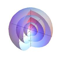
   nested spheres

   Find the radial mass density profile of the particles assuming that all particles have the same mass. For this step of the exercise just assume each particle has mass=1 (never mind the units). Recall the definition of density. When you made your histogram you used radius. So think about the 3D shape of each “bin” and how you would find its volume. Your density should be in units of (Mass unit)/kpc^3. Make sure your plots have axes labels.                                

6. Go back and redo steps 4 and 5 with log_10 (radius) instead of radius.  Notice how the histogram and density profiles change. An advanced exercise is to find the slope of the inner and outer parts of the profile when it is plotted in log-log space.
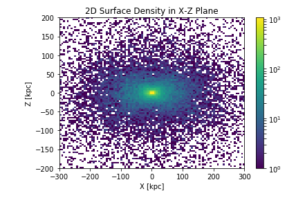
7.  Plot the 2-D surface density (projected density) either as a contour plot, grey scale or 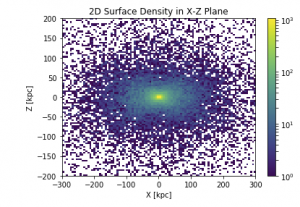color scale. Bin the particles on a 2D square grid in projection (x vs. y) or (x vs. z), the scale should be in units of Mass unit/kpc^2. Your plot should look something like the plot on the left.
8.  Find the absolute value of the 3 dimensional velocity (V_3d)  and make a scatter plot of V_3d versus radius. The upper envelope of this scatter plot is the escape velocity curve.
9. The formula for escape velocity at a distance r from the center of an object of mass M is given by V_esc = sqrt(2GM/r).  For an extended object like a galaxy the real formula for escape velocity is more complicated (and depends on mass beyond radius r). However let us approximate the escape velocity by V_esc ~ sqrt(2G M(r)/r) where M(r) is the mass enclosed in a radius r. As you get further and further from the center, this approximation will become closer and closer to the true value.
10. Compute the escape velocity  curve as a function of radius for this galaxy: use G = 4.35e-6. This is what  your standard G= 1.67e-8  becomes when you convert mass from kg to solar masses (1 solar mass = 2e+30kg), distance from meter to kpc and velocity from m/s to km/s). At first assume that each particle has 1M solar mass (i.e. give it mass=1). You will notice that with Mass unit = 1Msun the curve you get with the formula is much lower than the upper envelope of points in the scatter plot. So this should tell you that the particles don’t have mass=1 and you need to change the mass to make the curve go higher. So go ahead and change your mass per particle first by a factor of 10, then 1000. What happens to the curve? Keep going –  approximately what mass does each particle in the simulation need to have to ensure that the computed escape velocity at large radii from the center matches the upper envelope of points in your plot of V_3d vs. radius. (Yes it’s big!) With this particle mass what  do you estimate for the total mass of the simulated galaxy?
11. (Optional but recommended)  Write a 2 page summary of what you did this is exercise and what you learned from it. Feel free to include any plots that you generated.

Disclaimer/More details for professionals: This simulation is not actually that of an elliptical galaxy. It is extracted from a simulation of an isolated triaxial NFW dark matter halo created from the sequential merger of four NFW halos (Debattista et al. 2008). Also the original simulation had several million particles of which only about 40K have been randomly selected here. Nonetheless it’s possible to compute the total mass of the NFW halo from these data.