
This is a Graphical User Interface (GUI) addition to MATLAB scripts (here) that were published recently (PDF). This installer does not require one to have MATLAB, it will install the required MATLAB libraries automatically (downloaded from the web).
The installer can be found here: ITCFittingGUI along with example dataset that can be loaded to check out the features of the program.
Step 1: Load your ITC dataset
Text file saved from ITC, see xyz.DAT from here to obtain the correct format being read.
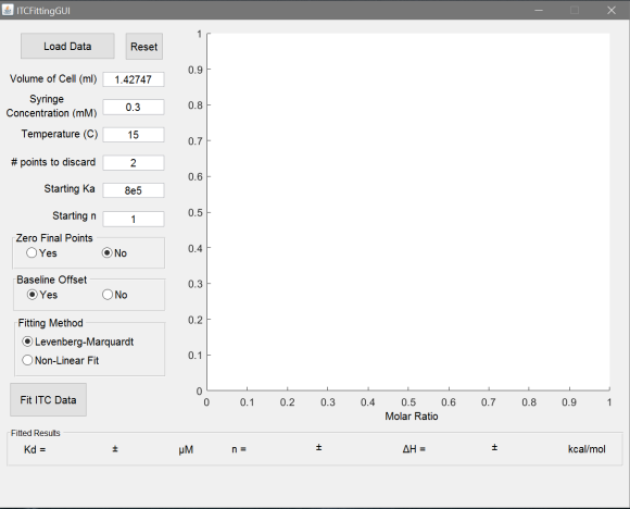
Step 1.1: Open the ITCFitGUI program
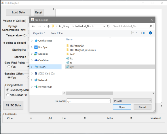
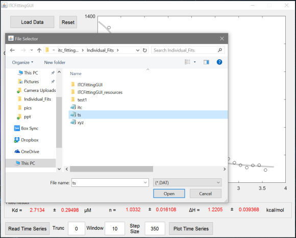
Step 1.2: Read the Data file (xyz.DAT)
Click on “Read ITC Data” Button in the top left corner and select appropriate ITC data file.
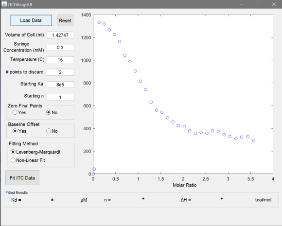
Step 1.3: Look for the Data on the right panel
Step 2: Fitting the Data
- Fill in the appropriate values for volume of sample cell, syringe concentration, temperature, number of initial points to discard, starting values of Ka and n. Please note that these vary from instrument to instrument and also between experiments on the same instrument. Remember to use correct values and not approximates.
- In “Zero Final Points”, choose between yes and no if one wants to make the last few points in the ITC experiment to be zero. This is a common practice for most ITC experiments where reference subtraction is not accurate.
- In “Baseline Offset”, choose between yes and no to automatically adding an offset in your fits. This can be activated if one does not want to make their final points in the ITC experiment zero from the previous option.
- Choose between Levenberg-Marquardt and Non-liner Prediction algorithms for fitting your ITC data.
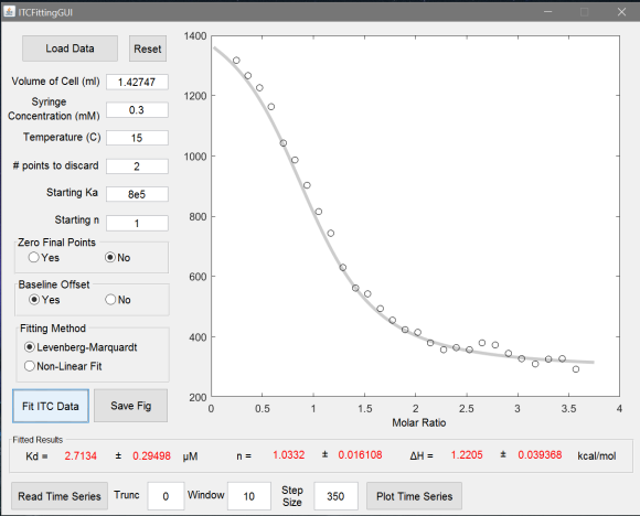
Save the figure by clicking “Save Fig” and note the fitted values in “red“.
Step 3: Plotting the Cp vs Time data
Some publications require the user to also present the raw injection data along with the fits. The lower section is used just for that purpose.
Step 3.1: Load the time-series data
Read the appropriate injection time series file. See ts.DAT from here to obtain the correct format being read.
Step 3.2: Adjust the baseline correcting parameters
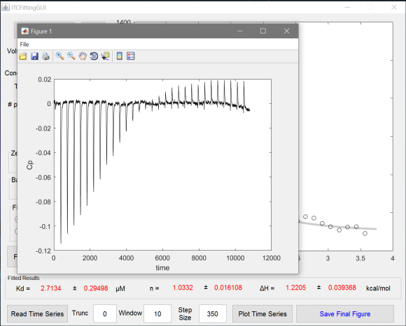
Once one gets satisfactory baseline correction for the ITC time-series, save the figure by clicking “Save Final Fig” in the bottom right corner.