Complete Active Space Self Consistent Field (CASSCF) in MOLPRO

CASSCF is a multiconfigurational method used to generate qualitatively correct reference states of molecules. Particularly useful when

• Hartree–Fock and density functional theory are not adequate e.g., for molecular ground states which are quasi-degenerate with low lying excited states or in bond breaking situations.
• Computing excited states for small-medium molecular systems. The energies are accurate within 0.1-0.2 eV, when a proper CASSCF reference wavefunction is employed as reference function for a subsequent treatment of dynamic correlation (e.g. CASPT2), which is an error bar sufficient for many spectroscopic applications.

In a CASSCF calculation, the set of coefficients of both the determinants and the basis functions in the molecular orbitals are varied to obtain the total electronic wavefunction with the lowest possible energy.

Basics on how to do a CASSCF computation:
1. Determine what orbitals to put in the active space.

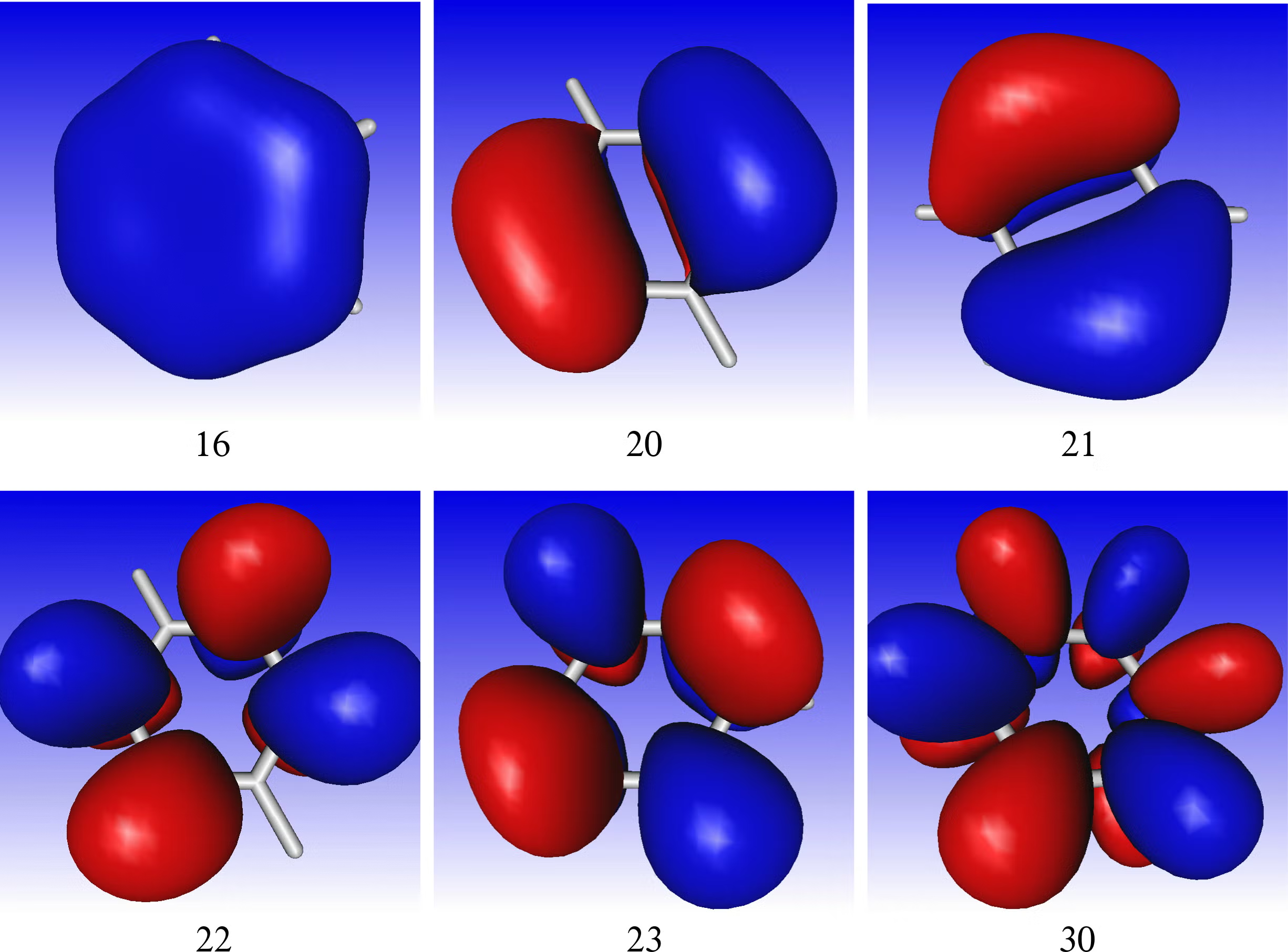
Compute the orbitals of the molecule at the HF level and visualize the orbitals using gmolden. Can also compute other orbitals such as natural bond orbitals (NBO), or natural orbitals. NBOs to be particularly helpful when the HF orbitals are very delocalized.
Choosing the active space orbitals is up to the user. For very small systems we can do all valence electrons. Unfortunately, this is not feasible for all molecules and reductions in the active space must be made (upper limit is 16 electrons in 16 orbitals). In the case of benzene, we only chose the pi-orbitals. In the case of reactions it is necessary to include all orbitals involved in the transformation. In the computation of high energy excited states, the valence states are usually interleaved with Rydberg states. Therefore, the active space has to include the necessary valence and Rydberg orbitals. That topic is not discussed here.

2. Select the active space using the occ, closed, and rotate command in MOLPRO
Occupied orbitals contain 2 electrons in all configurations, and closed electrons contain 0 electrons in all configurations. The difference between closed and occ, determine the number of active space orbitals.
To rotate the correct orbitals into the active space use the rotate command.

Sanity checks:
In order to check if the CASSCF calculation has been successful there are a number of tests that can be made.

• The energy converges.
• Orbital occupation numbers (diagonal elements of the density matrix) are not very close to zero or two (within three decimal places roughly). For the above calculation the occupancies are 1.95,1.87,1.87,0.13,0.13,0.05.
• Localize the orbitals. The orbitals should localize onto atomic sites and can be checked with a gmolden to verify that they are the correct orbitals to include in the active space.
• Good practices
  Save permanent file .wfu – Can be used to restart calculations and for future calculations, e.g. geometry optimizations, reduction in active space, etc.
• Want to know what configurations (think excitations) contribute to your state? Print the CI vector. This is always suggested because states can switch their order and be in an incorrect order; e.g. S1 can be a doubly excited state when it should be a singly excited state.
• Want to characterize the excited states in an intuitive way? Localize the orbitals and calculate the spin-exchange density matrix elements Pij (αβ terms) and occupation numbers (diagonal elements of the one-electron reduced density matrix). (Implemented in future tutorial).